Base stealing decisions are a very key element in gaining an edge over the opponent in tight games. Imagine a 1-1 game where both starting pitchers are carving up the opposing offenses. Your team finally gets another base runner on in the 7^th inning with one out. Who knows, maybe this is one of the last opportunities you’ll get to score, based on the climate of the game. Suddenly, the decision to steal second base becomes a crucial point.

Imagine that base runner has mediocre speed and agility. The decision becomes very risky. One the one hand, the swing in expected runs scored from runner on first with one out to runner on second with one out, is significant (+.15 in expected runs), especially in a one run game. On the other hand, the swing in the opposite direction from the current situation to no runners on with two outs is more extreme, a -.3 decrease in run expectancy. In this high leverage situation, it’d be convenient to have a visual decision guide handy to reference expected values of an attempt (accounting for probabilities of success and failure for that runner, and expressing recommendations in run expectancy changes).

I was curious to find a way to create an information system that can be used by managers and base coaches to facilitate their base stealing decisions, using an expected value framework.

In my first try at expressing this, I grabbed the career steal %s for each player, and used this formula to gather the expected run value of a steal attempt for each player:

              (Player Steal %) * (Delta Run Expectancy if Steal) + (Player Caught Steal%)*(Delta Run Expectancy if Caught)

I also added a percentage point to the players steal % for each percentage point the opposing catcher was below 30% CS.

The result was the following chart:

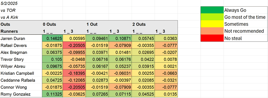
The interpretation of the numbers is as follows: The team’s gain in run expectancy is .146 on a Jarren Duran steal attempt of second with 0 outs and no other runners (and vs Alejandro Kirk). The change in run expectancy on a Connor Wong steal attempt of second with a runner on third with 2 outs is -.07 (not recommended worth the risk to steal).

To make the probability model more accurate, I would conduct a random forest classification. RF models use a variety of inputs to construct many decision trees that classify groups of observations as successful steals or unsuccessful steals. The decision trees are averaged to create the random forest model.[1]

The features I would utilize to construct these trees are pitcher handedness, catcher pop time, runner sprint speed, and player steal %. Along these dimensions, the decision trees would identify along which values a steal occurs on average.

To boost ability to generalize, I’d toggle with different settings for the max depth of the decision tree and the minimum leaf node size (cross validation of test sets on each setting). After landing on the parameters, the model outputs a probability of a successful steal. Then I would use those estimates to re-create the table!

---

[1] Each decision tree based on a random sample of the full data set. Data set compiled as a blend of retrosheet box score files (for stolen base attempts) and statcast data for tracking metrics.